
Shading under a distribution curve (eg. normal curve) in excel
We discussed on creating normal distribution curve in previous blog post. Please follow the same steps to create curve.
Here we need some more calculations to find the truncation point to shade the curve.
Let's say we want to have 50% (shaded) and 25% clear in both left and right.
| LeftClearEnd | 0.25 |
| RightClearStart | 0.75 |
Thus corresponding point for shading start and end will be:
Formula:
Shade left:
= NORMSINV($F$6)*$F$1 + $F$2
Shade Right:
=NORMSINV(F7)*$F$1+$F$2

Now we need to filter the data to be shaded fromt the total data used to plot the normal density curve (column Normal(Freq)). Thus for our middle shaded plot, the formula to calculate would be:
=IF(H2<$F$10,NA(),IF(H2>$F$11,NA(),I2))
Apply the formula, then you can see the filter value between ShadeLeft and ShadeRight will be preserved others will be turned to "#NA".
(1) Plot the density curve.
(2) Add new curve based on the "To be shaded (middle)" column

(3) Now we need to add error bars to the newly plotted series. Click the layout menu, then click add error bars and then more options, see the settings in the following figure.

(4) Remove the cap lines and slect the series and increase size of lines so that it fills the area. Chage color you like. A large number of bins are preferred as they will fill the area with out too much strech at boarder, which might make area shaded inaccurate by expanding out of trunication point.
(5) Hide the newly added line series by no line under Format Data series > Line color.

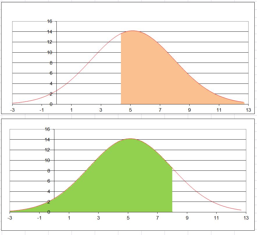
Shading left or right of any point can be done similar fashion. The only difference is the formula:
The formula for selecting right:
=IF(H2<$A$11,NA(),I2)
The formula for selecting left:
=IF(H2>$A$12,NA(),I2)
Best solution on the web, thanks!
ReplyDelete